Module 2: The Mathematics of Forecasting
Duration: 60 minutes
Learning Objectives
By the end of this module, you will be able to:
-
Understand why linear CPU/Memory trending fails for microservices architectures
-
Calculate "Pod Velocity" using Prometheus metrics
-
Build custom forecasting dashboards in Red Hat Advanced Cluster Management (RHACM)
-
Project quarterly node requirements based on deployment patterns
Why Linear Models Fail
Traditional capacity planning uses linear extrapolation:
If CPU usage grows 5% per month, in 12 months we'll need 60% more CPU.This breaks for microservices because:
-
New services deploy in bursts (not linear growth)
-
Resource requests vary wildly per service
-
Seasonal traffic patterns create spikes
-
Deployment velocity (new pods/month) matters more than raw CPU trends
The Pod Velocity Model
Instead of tracking CPU percentage, track how many pods are being deployed over time:
Pod Velocity = Rate of pod creation over timeIf your organization deploys 50 new microservices per quarter, and each requires an average of 3 replicas with 200m CPU each, you need:
50 services × 3 replicas × 200m CPU = 30,000m CPU (30 cores) per quarterThis is far more accurate than linear CPU trending because it accounts for workload growth patterns.
|
The Formula: Example: - Pod Velocity: 50 new services/quarter - Avg Replicas: 3 - Avg CPU Request: 200m (0.2 cores) - Node CPU: 8 cores allocatable Round up → You need 4 new worker nodes every quarter. |
Lab 2: The Pod Velocity Calculator & ACM Dashboard
|
All terminal commands in this lab run on your student cluster. If your SSH session ended, reconnect before continuing: SSH password: |
In this lab, you’ll use purpose-built scripts to query Prometheus directly from the command line, run the forecasting formula automatically, and create a centralized RHACM dashboard — without having to navigate any browser UIs until the final step.
Download Lab Scripts
Download both lab scripts at the start. They are used throughout this module.
mkdir -p ~/module-02 && cd ~/module-02
BASE=https://raw.githubusercontent.com/tosin2013/capacity-planning-lab-guide/main
curl -fsSO $BASE/content/modules/ROOT/examples/module-02/pod-velocity-calculator.sh
curl -fsSO $BASE/content/modules/ROOT/examples/module-02/create-acm-dashboard.sh
curl -fsSO $BASE/content/modules/ROOT/examples/module-02/module-2---pod-velocity-forecast.yaml
chmod +x *.sh
ls -lh-rwxr-xr-x. 1 lab-user lab-user 11K Apr 20 create-acm-dashboard.sh
-rw-r--r--. 1 lab-user lab-user 4.2K Apr 20 module-2---pod-velocity-forecast.yaml
-rwxr-xr-x. 1 lab-user lab-user 8.8K Apr 20 pod-velocity-calculator.shPart 1: Run the Pod Velocity Calculator
The pod-velocity-calculator.sh script does everything Parts 1-5 used to require of you manually — it discovers Prometheus automatically, mints an auth token, runs all four PromQL queries, and prints the forecasting result.
cd ~/module-02
NAMESPACE=capacity-workshop ./pod-velocity-calculator.sh══════════════════════════════════════════════════
Module 2 — Pod Velocity Calculator
══════════════════════════════════════════════════
[INFO] Namespace : capacity-workshop
[INFO] Window : 30 days
[INFO] Node CPU : 8 cores (allocatable)
[INFO] Step 1/5 — Locating Prometheus route …
[OK] Prometheus : https://prometheus-k8s-openshift-monitoring.apps.student.student-01.sandbox5388.opentlc.com
[INFO] Step 2/5 — Minting Prometheus service-account token …
[OK] Token acquired (1287 chars)
[INFO] Step 3/5 — Calculating pod velocity …
[OK] Pods started in last 30d : 6
[OK] Pod velocity : 0.2 pods/day
[INFO] Step 4/5 — Querying average resource requests …
[OK] Active deployments : 6
[OK] Avg replicas per deployment : 1.0
[OK] Avg CPU request per container : 167m (0.167 cores)
[OK] Avg Memory request per container: 192Mi (0.188 GiB)
┌─────────────────────────────────────────────────────┐
│ QUARTERLY FORECASTING MODEL │
├─────────────────────────────────────────────────────┤
│ Pod velocity (last 30d) : 0.20 pods/day │
│ Quarterly new pods (×90) : 18.0 │
│ Avg CPU request/container : 167m │
│ Total CPU needed (new) : 3.01 cores │
│ Node allocatable CPU : 8 cores/node │
├─────────────────────────────────────────────────────┤
│ Nodes needed next quarter : 0.38 → ceil = 1 │
└─────────────────────────────────────────────────────┘
RESULT: Add 1 worker node(s) this quarter to accommodate forecasted growth.|
Understanding what the script queries:
Want to see the raw PromQL? Open |
Part 2: Interpret Your Numbers
Look at the output from the calculator. Answer these questions for your own environment:
| Metric | Your Value |
|---|---|
Pod velocity (pods/day) |
|
Quarterly new pods projected |
|
Avg CPU request per container |
|
Nodes needed next quarter |
|
Forecasting Pitfall: This model assumes deployment cadence stays constant. It will overestimate if your cluster is still being bootstrapped (many deployments all at once), and underestimate during growth phases. Always combine model output with team-level deployment plans. |
Part 3: Adjust for Your Node Size
Rerun the calculator with the actual allocatable CPU for your worker nodes:
NODE_ALLOC_RAW=$(oc get node -l node-role.kubernetes.io/worker \
  -o jsonpath='{.items[0].status.allocatable.cpu}')
# Convert millicores (e.g. 7500m) to cores (7.5); leave whole-core values unchanged
NODE_ALLOC=$(python3 -c "
v='$NODE_ALLOC_RAW'
if v.endswith('m'):
    print(round(int(v[:-1]) / 1000, 2))
else:
    print(round(float(v), 2))
")
echo "Worker node allocatable CPU: $NODE_ALLOC cores"
Then rerun with the real value:
cd ~/module-02
NAMESPACE=capacity-workshop NODE_CPU=$NODE_ALLOC ./pod-velocity-calculator.sh
Compare the "Nodes needed" figure to the default (8-core assumption). Does a larger node size reduce your projected node count significantly?
Part 4: Publish the Pod Velocity Dashboard to RHACM Grafana
Push the forecasting panels into the RHACM Grafana instance running on the hub cluster.
You will switch your oc context to the hub, apply a pre-built dashboard ConfigMap, then switch back — a pattern you will reuse in Module 5.
|
Why switch context? RHACM Grafana runs on the hub cluster. Your current |
Step 4a — Save your student context and log into the hub
STUDENT_CTX=$(oc config current-context)
echo "Student context saved: $STUDENT_CTX"
oc login  \
  --username= \
  --password= \
--insecure-skip-tls-verify=trueStudent context saved: capacity-workshop/api-student-student-01-sandbox5388-opentlc-com:6443/system:admin
Login successful.
You don't have any projects. You can try to create a new project, by running
oc new-project <projectname>Step 4b — Apply the Pod Velocity Forecast dashboard ConfigMap
oc apply -f ~/module-02/module-2---pod-velocity-forecast.yaml \
-n open-cluster-management-observabilityconfigmap/module-2---pod-velocity-forecast createdThe grafana-dashboard-loader sidecar detects the new ConfigMap (labelled
grafana-custom-dashboard: "true") and imports it into production Grafana
within a few seconds.
Step 4c — Switch back to your student cluster
oc config use-context $STUDENT_CTX
oc whoamiSwitched to context "capacity-workshop/api-student-student-01-sandbox5388-opentlc-com:6443/system:admin".
system:admin|
This three-step pattern — save context, login to hub, switch back — is used again in Module 5 when you import your student cluster into RHACM. |
How RHACM Dev Grafana Works
The ConfigMap you just applied was generated using the official RHACM Development Grafana tooling from the multicluster-observability-operator repository. Understanding this workflow is useful when you want to build your own custom dashboards in a real environment.
A Dev Grafana instance is already running in this workshop hub at:
Log in with your hub credentials ( / ) and explore freely — it connects to the same Thanos datasource as production Grafana but gives you full editor access in the UI.
The interactive dashboard workflow
When you want to create or modify dashboards from scratch:
-
Deploy Dev Grafana (hub admin runs once):
git clone --depth 1 \ https://github.com/stolostron/multicluster-observability-operator.git ~/acm-tools cd ~/acm-tools/tools bash setup-grafana-dev.sh --deploy -
Log into Dev Grafana in your browser — this creates your user record in the Dev Grafana database, which the export script requires.
-
Promote yourself to Grafana Admin (optional — needed to create/save dashboards):
bash switch-to-grafana-admin.sh -
Design your dashboard in the Dev Grafana UI. Create a folder named after yourself, build the panels, and save. The Thanos datasource with all managed cluster metrics is already configured.
-
Export to a production ConfigMap:
bash generate-dashboard-configmap-yaml.sh "Your Dashboard Name"
# To target a specific folder:
bash generate-dashboard-configmap-yaml.sh -f "Your Folder" "Your Dashboard Name"
The exported YAML is labelled
grafana-custom-dashboard: "true"and optionally annotated withobservability.open-cluster-management.io/dashboard-folder: <folder>— the loader uses this to place the dashboard in your named folder in production. -
Apply to production Grafana:
oc apply -f your-dashboard-name.yaml -n open-cluster-management-observability -
Clean up Dev Grafana when done:
bash setup-grafana-dev.sh --clean
|
|
Part 5: Log In to Grafana and View the Dashboard
Step 5a — Open the dashboard URL
Open a new browser tab and navigate directly to the RHACM Grafana instance:
Once logged in, browse to Dashboards → Custom → Module 2 — Pod Velocity Forecast.
|
You can also use the direct dashboard URL:
|
Step 5b — Authenticate with OpenShift
RHACM Grafana uses OpenShift OAuth — there is no separate Grafana username or password to set up. Follow these steps on the login page:
-
Click Log in with OpenShift.
-
On the OpenShift login page, choose the workshop-students identity provider.
-
Enter your hub credentials:
Field Value Username
Password
-
Click Log in — you are redirected back to Grafana automatically.
|
The identity provider is named workshop-students because the hub cluster was configured with an htpasswd provider for all student accounts. If you see other providers (e.g. |
Step 5c — Explore the dashboard panels
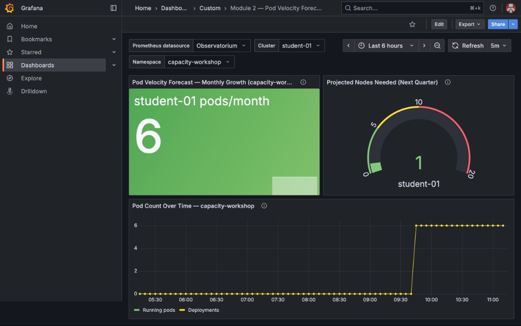
Once logged in you will see three panels:
-
Pod Velocity Forecast — Monthly Growth (capacity-workshop) (Stat panels, one per cluster) — pods started in
capacity-workshopin the last 30 days; should match the "Pods started in last 30d" value frompod-velocity-calculator.sh -
Projected Nodes Needed (Next Quarter) (Gauge panels, one per cluster) — the computed node requirement with green/yellow/red thresholds; should match the "Nodes needed next quarter" from the script
-
Pod Count Over Time (Time series) — a historical view of pod growth in
capacity-workshop
|
What to look for:
Because |
|
The Cluster and Namespace dropdowns default to Now change Namespace to All — notice how the numbers jump: |
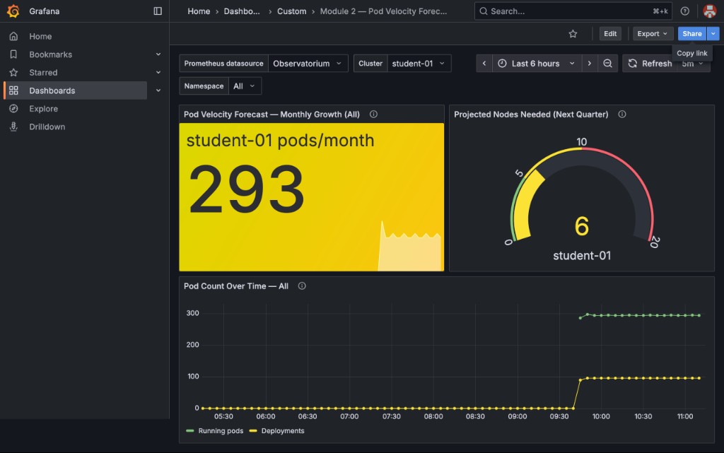
|
This is why namespace scoping matters in capacity planning. Those 293 pods are every OpenShift platform pod (etcd, API server, monitoring, DNS, etc.) started when the cluster was provisioned. Unscoped, the model recommends 6 new nodes for workloads that are already running and won’t grow. Always scope your velocity query to the namespaces your application teams control. |
Part 6: Validate the Forecast
Let’s cross-check the model against what’s actually running. Run this command to count current pods:
oc get pods -n capacity-workshop --no-headers | wc -lNow run the full validation echo:
echo "Current pod count: $(oc get pods -n capacity-workshop --no-headers | wc -l)"
echo ""
echo "Forecast predicted (based on 30-day velocity):"
echo "This would require manual calculation from historical data"|
Facilitator Discussion Point: In production, you’d store daily snapshots of these metrics in a time-series database (Thanos/Prometheus long-term storage) to validate forecast accuracy over time. Accuracy improves with:
|
Lab 2 Summary: Your Forecasting Model
You’ve now built:
✅ Pod Velocity calculation using the Prometheus API (no browser PromQL needed) ✅ Average resource request metrics pulled automatically ✅ Quarterly node requirement projection formula ✅ Custom RHACM Grafana dashboard for fleet-wide visibility — published via ConfigMap ✅ Understanding of why Pod Velocity beats linear CPU trending
Real-World Application
Take this model back to your organization:
-
Capture your deployment cadence - How many new services per quarter?
-
Measure average resource requests - What’s your "standard microservice footprint"?
-
Calculate node runway - When will you run out of capacity?
-
Build forecasting into your change approval process - Every new service deployment should update the forecast
|
Reusing these scripts in your own environment: Both scripts accept environment variables so you can adapt them without editing: The scripts are designed to be run repeatedly — |
|
The Forecasting Pitfall: Forecasting is only as good as your resource requests. If developers over-request by 10x, your forecast will tell you to buy 10x more hardware than you actually need. This is why Module 3 (Developer Track - Right-Sizing) is critical. You must fix request accuracy BEFORE forecasting, or you’ll forecast waste. |
Key Takeaways
-
Pod Velocity (deployments/time) is more predictive than linear CPU trending for microservices
-
The Prometheus API lets you query PromQL from scripts — no browser UI required
-
RHACM provides fleet-wide capacity visibility across multiple clusters
-
RHACM Dev Grafana provides a full-editor instance for interactive dashboard creation — export with
generate-dashboard-configmap-yaml.shand promote to production via ConfigMap labelledgrafana-custom-dashboard: "true" -
Forecasting accuracy depends on accurate resource requests (Module 3 fixes this)
Next Steps
In Module 3: Developer Track - The "Zero Request" Myth, we’ll tackle the root cause of forecasting inaccuracy: incorrect or missing resource requests. You’ll learn about QoS classes, debug throttling, and right-size workloads using historical Prometheus data.
|
Pre-Module 3 Setup: We’ve pre-deployed sample applications in |